
An intro to the Tensor Economics blog
An excellent blog on LLM economics, with reference to related work by SemiAnalysis.

The Tensor Economics blog covers the economics of producing text from language models at scale.
The posts themselves are wonderfully detailed but somewhat overwhelming. I want to provide a summary of their work that might act as a guide. Then I’ll tie in some complimentary data from SemiAnalysis.
Note that I am presenting their posts in a different order to make it flow better. Each section selects a small amount from each of the original posts. Ideally, this post gives you the scaffolding to read their posts in full, they have a lot more insight.
Preludes
Time is money
Roughly 50% of AI data center spending is on hardware. Other CapEx1 grows in proportion to hardware costs2.
Hardware depreciates in value (and there are loans to pay off), so you need it to produce as many valuable tokens during its lifetime as possible. Naturally, our emphasis will be on the speed a GPU (and the supporting equipment) can do things.
Let me be clear about what it means for a GPU to depreciate. While GPU’s can slow down, or get more faulty, or break, the primary source of depreciation is obsolescence. Nvidia keeps making faster GPU’s. These are more expensive, but the higher speed counteracts the price and the overall cost per token is lower. At some point it makes sense to swap out your old (still functioning) GPU for a new one.
Defining some units
FLOP means “floating point operation”, such as an add or multiply. However, “FLOPs” and “FLOPS” are completely different units. FLOPs is merely the plural of FLOP, while FLOPS means FLOP/s. This is very dumb.
Most places assume people understand the difference. But clarity matters!
I’m going to use FLOP as plural (i.e. FLOP=FLOPs) and write FLOPS as FLOP/s. This is different than most texts but easier to understand in my opinion.
The rest of the units we will use are more clear. Memory bandwidth and communication speed are measured in gigabytes per second or GB/s. We will talk about “tokens” a lot (see next section) which I’ll shorten to “tok”. One million tokens is “Mtok”.
How transformer inference works
Instead of a full explanation, I’ll highlight a few things and point to others who have explained it better. It’s not critical that you know this stuff, but I want this post to be self-contained.
Language models process tokens, which aren’t quite words, more like “wordlets”. The image below illustrates this nicely. Essentially, you break a text down into a sequence of tokens from a pre-defined list. You can then associate each possible token with an index on this pre-defined list.

The next step is to take this list of input (prompt) tokens and in some sense embed the input into the LLM activations. Specifically, you do a forward pass through the transformer, applying the attention operation and feed forward blocks to the tokens in the prompt. This phase is called prefill or prompt-processing. It comes before the transformer can produce the first token of its response.
The attention operation applies to all pairs of tokens in the prompt and ensuing response. You can save a lot of computation by storing the results of the attention operation applied to pairs of tokens in the prompt. That way, each new token only needs to interact with previous tokens, you don’t need to re-do the attention operation for pairs of tokens you’ve already seen.
This store of previous attention results is called the KV cache. The details aren’t too important, but you should know that:
The KV cache is large enough that it needs to be stored in HBM and streamed in to the GPU as needed.
Longer prompts and longer LLM responses require a larger KV cache.
A separate KV cache is required for each prompt. In other words, if you have 10 user requests, you need to store 10 KV caches.
Typically the KV cache is much smaller than the weights of the model.
This discussion has glossed over a lot of details. It’s not necessary for this post, but to understand LLM inference from a high level, I recommend starting at this video in a 3blue1brown series on deep learning. One caution is that the specific way attention is done and the overall architecture of leading LLM’s continues to change, but the basic ideas are there.
This post from Tensor Economics covers inference in Llama 3 in more detail.
Weights must load from global memory creating two phases
There’s a tradeoff with memory: it can either be cheap or fast. There’s a whole memory hierarchy between small/fast/expensive memory and big/slow/cheap memory.
Some types of memory are located close to the processing center of the GPU. This memory can be accessed quickly, but it doesn’t have much capacity. It would be expensive to build more into the chip.
You can put lots of memory outside the chip for much lower cost, but this will be much slower. Even at light speed, small distances from the chip make memory access much slower.
Modern AI hardware has a large amount of off-chip memory located close to the GPU with a high-bandwidth connection to the chip. This is called high-bandwidth memory (HBM)34.
To actually do inference, you need to load portions of the model from the HBM into the GPU itself for calculations. That takes precious time. So there inference can be divided into two phases, a memory-bound phase where you wait for the weights to load, and a compute-bound phase where you do the actual computations. This is the key insight from which the next few sections derive.
FLOP/s/$: embeddings and the compute-bound phase
Why are embeddings so cheap? looks at the process of generating an “embedding” for a piece of text. Embeddings convert a document into a vector storing semantic information about the document. They’re a key part of using LLM’s to search for relevant text.
Inference providers like OpenAI charge $60 per 1M output tokens, while embeddings cost 10 *cents* to process 1M tokens. This is strange because (as we’ll see) inference and embeddings involve quite similar steps. Hence the question in the title.
Computing an embedding
Producing an embedding involves a single forward pass to load the document information into language model activations. These activations form the embedding.
The process of converting the document into activations is essentially identical to the prefill phase. So while embeddings themselves aren’t exciting, they give us some insight into the economics of LLM inference.
The compute-bound phase
We always need to load weights into the GPU and then run the actual computation. Which phase is the bottleneck?
Note that embeddings typically use a small-ish language model, less than 10B parameters. In the post, the authors offer a quick calculation based on a Qwen3-8B embedding.
So it takes almost 5x longer to do the computations as it takes to load the model from memory. So embeddings are primarily compute-bound. We want a chip that performs FLOP as fast as possible. In other words, we want hardware with a high FLOP/s/$.
The authors then do lots of benchmarking to show that this intuition is correct.
Why embeddings are so cheap
One last thing to understand why embeddings are so much cheaper than normal inference. All the embeddings provided by different companies converge to similar representations5. That is, their products aren’t differentiated from each other. That creates a lot of competition:
Our contention is that since the cost of processing a token is so minuscule and all embedding models converge to similar semantic representations, this means that no provider enjoys a sustainable moat. This results in underlying low costs being passed directly onto the consumers, driving prices to rock bottom.
That’s the key takeaway here. A few other interesting tidbits:
They look at actual hardware and estimate that the true cost of embeddings could fall almost 10x to around 2 cents per Mtok.
Interestingly, the real world performance (FLOP/s/$) of the RTX 4090 (older GPU) is better than an H100 (newer GPU).
The authors suggest that “[t]he embedding situation offers a nice pre-taste of the “intelligence involution” that is coming …”. Hinting that they think the same competitive dynamics will come for LLM inference.
GB/s/$: inference and the memory-bound phase
LLM Inference Economics from First Principles is a massive post. They use Llama3-70B as their guide for the discussion. It’s open-source, easier to understand, and much of the industry has standardized around it.
Storing Llama3-70B takes 141 GB, this is more than the ~80 GB of HBM found on typical hardware like an H100. So right off the bat, you’ll need to load the model across multiple GPU’s for inference.
The post goes into great detail on the FLOP required to do inference on this model. It’s a great reference, but beyond our scope.
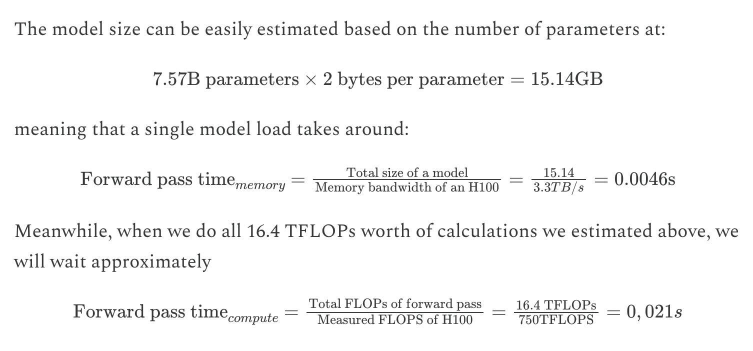
Equipped with an understanding of how many FLOP are required for inference, they estimate how long it would take to do prefill (prompt processing) for an input of 2048 tokens (~6 pages of double-spaced text).
To do the computations, it would take 0.29 seconds. To load the weights from HBM, it would take 0.04 seconds. The computations are the bottleneck, so the prefill phase is compute bound, just like with embeddings.
But prefill is just one step, what about actually generating output tokens? After a detailed discussion of the decoding (token-producing) phase, they give an estimate. It would take 0.00014 seconds to compute 2049 tokens of output. Yes, that’s the correct number of zeros.
So generating tokens is way, way faster than loading the weights from the HBM. This phase is primarily memory bound! That means you want hardware with a high memory bandwidth, FLOP/s isn’t as important for this phase.
They say:
... one of the insights we hope you take out of reading this article - the token-by-token phase is memory bound; the amount of available compute throughput is of secondary importance, as we massively underutilize the compute resources anyway while waiting for weights to be loaded.
They go into some nuances about what happens at longer input lengths and consider various tricks to run inference in parallel across GPU’s. Once again, out of scope. Instead, let’s look at the implications of being memory bound.
Batching
So no matter what, at each phase of inference, you need to load the parameters from that phase into the GPU and then do some calculations. Loading those parameters takes a fixed amount of time. Batching is the idea that, while the weights are loaded for that phase, you also perform the necessary calculation on another customer’s input6.
Imagine your job is to shred paper. You can either switch on the shredder and run it each time you get a piece of paper, or you wait until you’ve gathered a stack of paper, turn on the machine once, and shred a whole stack at the same time.
So batching waits for several customer requests and then runs inference on them all at the same time. There’s a fundamental tradeoff here: batching means that inference costs less money, but customers have to wait much longer to get their response. For example, batching 8 customers might cost 8x less and take 8x longer to get a response.
This is a big economy of scale for inference providers, the more customers you have, the lower price you can charge. Having more GPU’s to run inference in parallel helps too.
GB/s/$ matters
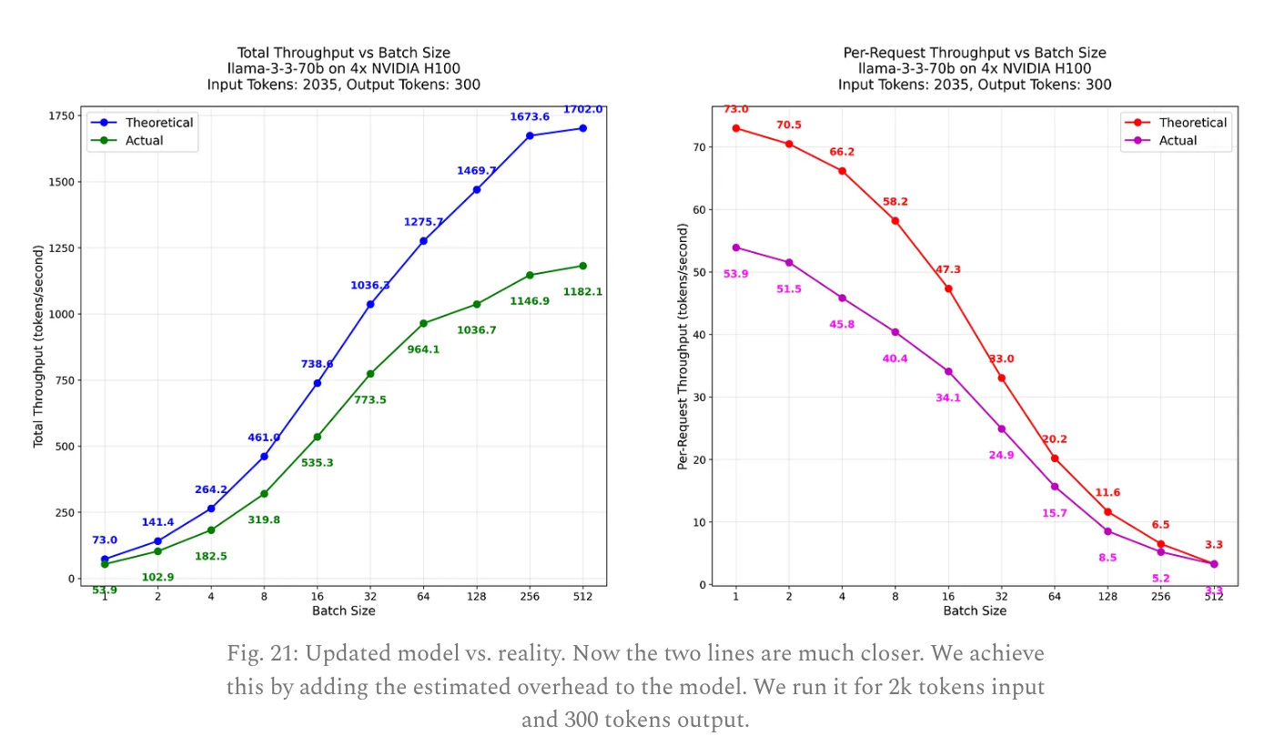
After all this, they run some benchmarks to show that their model lines up with reality. Real world inefficiencies make the true performance a little worse than you would expect.
Having a detailed model lets them estimate how much it would cost to run Llama3-70B on four H100’s: $1.72/Mtok. That’s 100x more expensive than computing an embedding, but much cheaper than the $60/Mtok of output that Open AI charges7. Though Open AI offers larger and more useful models than Llama-3 70B so the price may be justified.
Their post concludes by highlighting the importance of memory bandwidth for inference costs.
Interconnect and MoE inference
Now to the final post in our trilogy: MoE Inference Economics from First Principles. The last section was based on dense models like Llama3, but these have been replaced with mixture-of-experts (MoE) models. MoE models are typically larger but only activate a small fraction of their available parameters on each token.
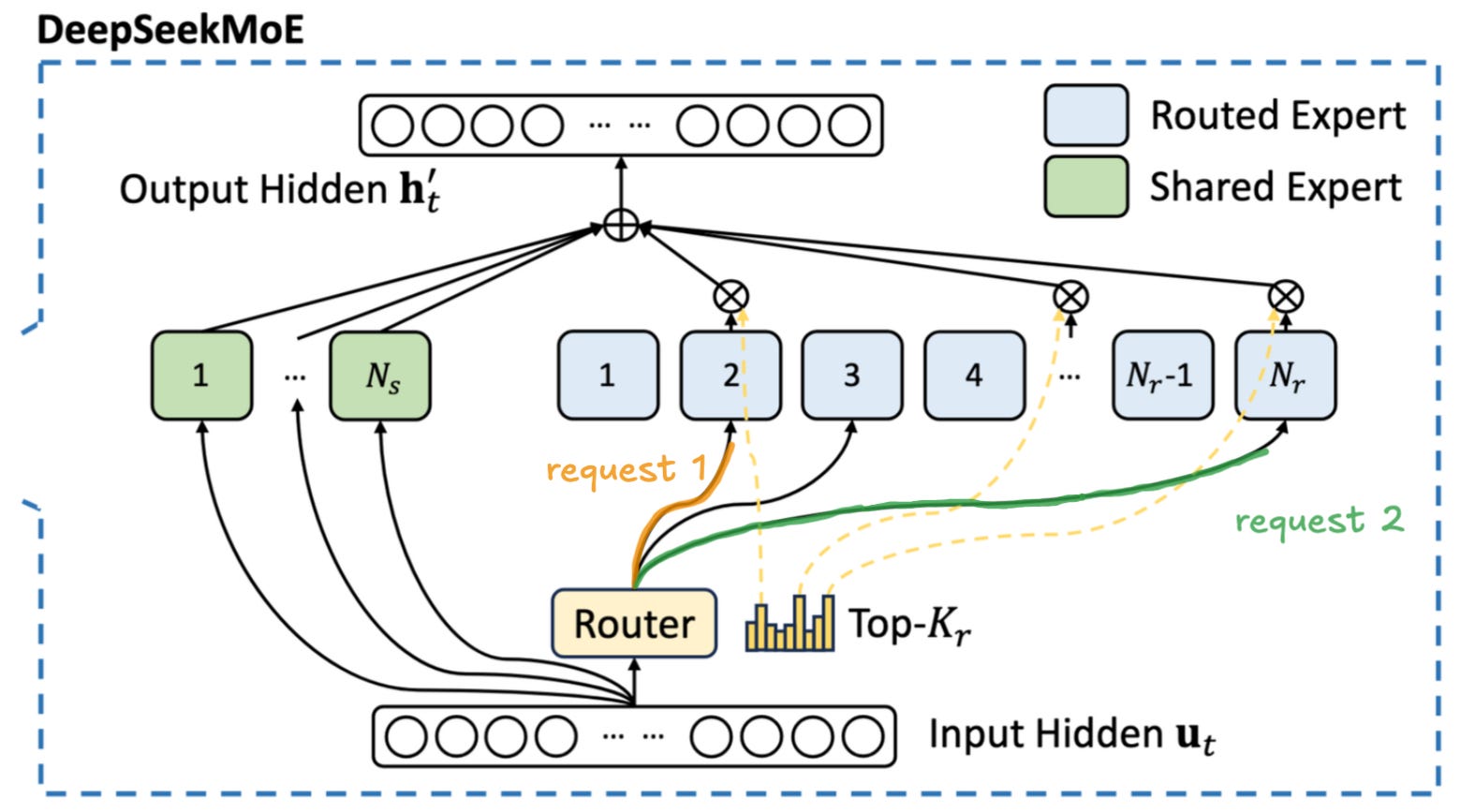
For this post, the authors focus on DeepSeek V3.1 which has 671B parameters but only activates 37B at a time.
With few parameters activated, you can be sneaky and only load the parameters you need for each token. As more users arrive, you need to load more and more of the model to a GPU. With enough users, you can load the whole model across GPUs and route requests through them.
So with MoE, you want more users and there are even bigger returns to scale with more GPUs. But since we’re routing requests between GPUs, we need high quality interconnections. Groups of GPUs with interconnections are called nodes.
Another benefit of scale: with MoE models needing more users, that will require more KV cache space. Moving all those Key and Value matrices around to other GPUs requires high memory bandwidth as well. It helps to have more GPUs and nodes to divide up the task of moving all this memory around.
They say:
Increasing the number of nodes operating within a single setup has a beneficial effect not only on the end-to-end performance but also on the per node performance.
... [A]s we increase the number of nodes involved (the EP number), the per node performance increases.
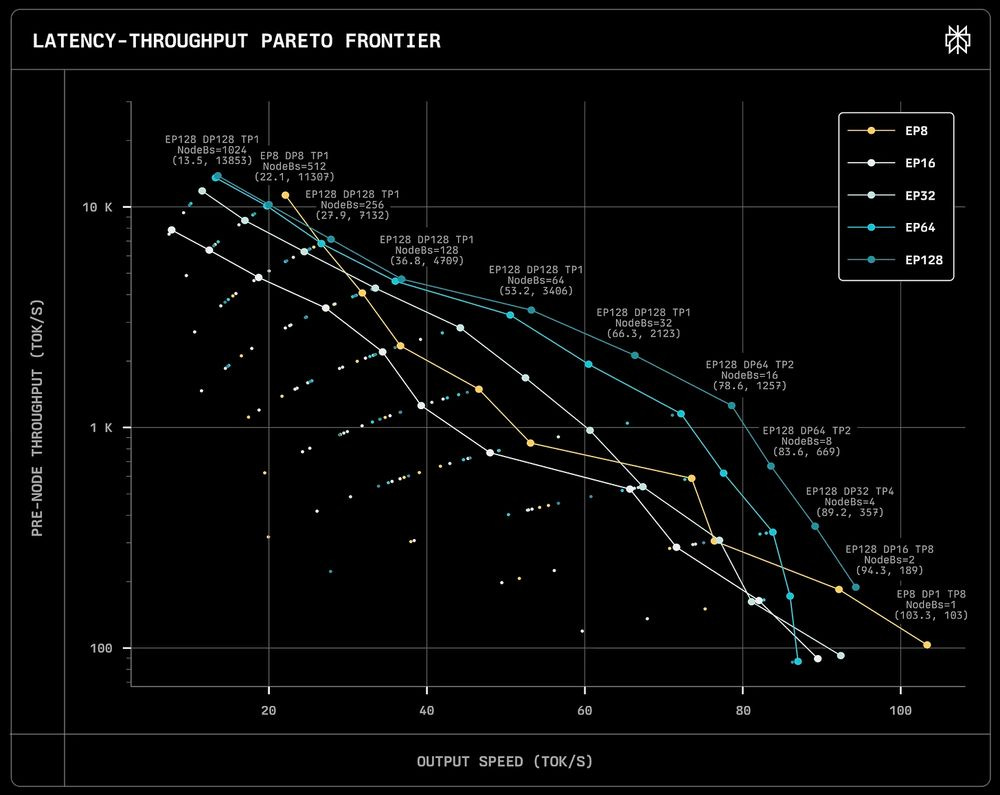
The chart above reiterates the fundamental tradeoff with serving LLM’s. Batching more users together means lower costs (i.e. higher speed per GPU) but also your users have to wait longer.
Next, they go into tons of detail on DeepSeek architecture, FLOP required for MoE inference, empirical data, etc. I’ll skip it and jump to the section “Hardware considerations and profit margins”.
Figure 24 confirms what we’ve been talking about, more GPU’s means more performance. Also, notice that switching from H100 to GB200 with fancy interconnects (that’s the NVL72 aka “NVLink”) gives a huge performance boost.
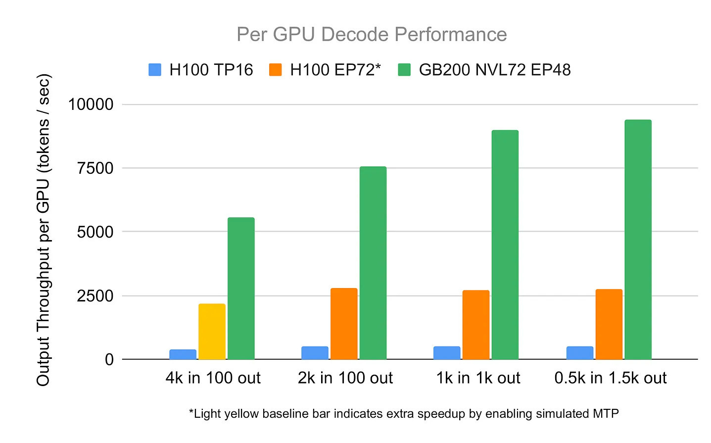
Indeed, the communication speed between GPU’s is super important. “There seems to be a massive performance gap between the numbers we estimate for B200s connected via InfiniBand and the ones connected by NVLink.”
In fact B200’s (newer GPUs) might not be worth it:
... [w]e believe that for model of a scale such as DeepSeek, running on B200s might be actually suboptimal, as the comms overhead is taking away most of the gains we get from faster memory and more FLOPS compared to H100s (see Fig. 27).”
So the key result from this post is that fast interconnections between your GPUs is crucial to properly utilizing your expensive hardware. You don’t want your expensive hardware waiting around for light to cross the room.
Other notes from this post
A few other interesting points in the final sections:
They observe is how “chat centric” most inference providers are, offering 50+ tok/s. “While this is great if we have real time application like a chat, it is less than optimal if we want to use the model to generate the synthetic data.”
They are LoRA-pilled and propose something similar to RLaaS:
Furthermore, to improve the inference economics, such RL models could be trained using LoRA adapters or a similar technique and served alongside thousands of other models, all catered to specific use cases. This multi-tenant serving approach represents a compelling business opportunity for inference providers. Clients hosting their custom LoRA adapters on a provider’s infrastructure face significant switching costs when migrating to competitors, as the adapters are optimized for specific serving configurations and client workflows. RLFT is based on unique and nuanced rewards that are very client-specific; unlike standard supervised fine-tuning (SFT), it much much more challenging to replicate it just via in-context learning, making it an even more compelling case for inference providers.
DeepSeek is the most popular model on OpenRouter. OpenRouter’s daily global consumption of DeepSeek is 1B tokens. They do the math and find that one
8xH100NVLink72 node could handle this demand 20x over.“How is it possible that the global consumption of the most popular open-source model is so small that it could be met by a single NVL72 with 20 times the capacity to spare? Given this low demand, how can so many inference providers sustain their businesses? Put simply: who is making money here?”
Very ominous! They suggest that perhaps the vast majority of DeepSeek demand is going directly to DeepSeek itself, despite the fact that it’s an open-source model (EDIT: they also suggest demand could be going primarily to other open-source providers like Fireworks or Together AI).
We find this dichotomy between Google, ByteDance, or MSFT declaring that they are processing trillions of tokens daily and the minuscule numbers we see for open-source providers to be quite perplexing!
Cross-checking with InferenceMax
Recently, SemiAnalysis released a dataset called InferenceMAX on the token economics of different types of hardware.
Their introductory blog post mentions a tradeoff we’re now familiar with:
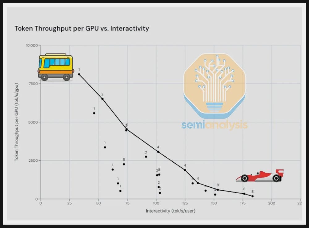
Playing around with their data portal, I think this is one of the key charts:
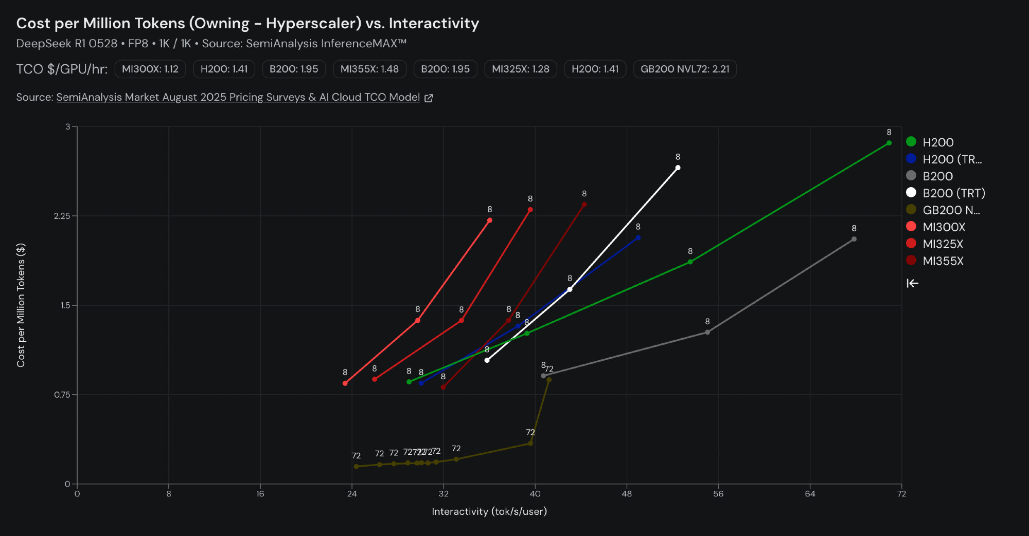
The tan line is GB200 NVL72. That refers to a node of 72 GPUs connected with NVLink72, a fancy interconnect. Notice how it achieves far lower costs (but not speed!) than the other options.
Notice that at high interactivity, the GB200 loses its edge, “... a single node B200 server can drive better TCO per performance than the GB200 NVL72 for high interactivity use cases.”
That’s because when you need to serve users quickly, you’re serving ~1 at a time. You lose the gains from scale from all those GPUs. All that interconnect adds cost without any benefit.
So InferenceMax confirmed some of the lessons from this post with a far more detailed cost model.
Main takeaways
The economics of LLM inference is fascinating. The Tensor Economics authors argue that “... the key question that will determine the profitability [LLM companies] can enjoy is the inference cost structure.”
These profits impact how accessible model is to consumers, feasibility of things like synthetic data, the amount of R&D companies can do. The future of AI is written in the economics of tokens!
I hope you get the following takeaways from this tour:
GPU’s are a big portion of overall LLM inference costs.
Newer generations of GPU’s have better overall cost per token despite higher prices8. That drives depreciation.
Because of depreciation, time is money. You need to utilize your GPU’s as much as possible before they become obsolete.
Utilizing your GPU’s a lot requires high processing speed. Two key speeds are FLOP/s and memory bandwidth (GB/s).
There are substantial returns to scale in LLM inference. More users means you can batch requests and lower costs. More GPUs unlocks parallel computation and higher memory bandwidth.
Getting these gains from scale requires high bandwidth interconnections between GPUs.
After all of this work, the authors come to the conclusion that inference markets will specialize:
We expect the inference markets to further specialize in regard to offered throughput, latency, and pricing. It is only natural for providers of super-fast tokens like Groq and Cerebras to command a much higher premium for the tokens they deliver at few-second latencies and for other providers like NeoCloud specializing in high-latency, high-throughput inference scenarios focused on synthetic data generation. We hope to elaborate on this space in the future text.
My thoughts
All this research focused on the transformer model, but many of these lessons would apply to a new architecture or approach. There will always be bottlenecks stemming from moving data and doing computations9.
Will hardware progress change the economics? That’s a topic for a future post, but note that rapid progress has mixed effects for inference providers. New chips produce tokens faster, but depreciate faster.
For the foreseeable future, returns to scale in inference will remain. Running LLM locally only makes sense if you want extremely low latency and are willing to pay a premium. On the other hand, distributed training only makes sense in the context of barriers to assembling compute.
Because you need enough capital to assemble all this compute, inference will naturally concentrate in a few players. The economics are also highly sensitive to interest rates. When rates are high, inference is expensive and few companies can serve models at scale.
For the companies that can assemble enough compute, the economics are pretty clear. There isn’t much secret sauce at the hardware level. Instead, they compete over the quality of the LLM they’re serving and the augmentations it has. I find the quality of frontier LLMs similar and expect competition to pivot to the augmentation level with RL-as-a-Service.
Edit: Piotr Mazurek (lead author of Tensor Economics) kindly responded to my request for feedback. I’ve incorporated some suggestions.
Racks, interconnect, cooling, energy infrastructure, buildings, construction labor, land.
What data center costs don’t grow directly with hardware cost? Water costs for cooling will depend on energy consumption, not hardware spend per se. If you’re using fossil fuel generators or nuclear plants, then the cost of fuel will grow in proportion to energy consumption (though fuel costs are dwarfed by CapEx for nuclear plants). Though I think off-grid renewables will make these energy sources all but obsolete for this application.
Note that the authors also call HBM “global memory” in their post.
A few more notes on memory:
HBM uses a fast memory technology called DRAM that needs to constantly be refreshed. This is because DRAM memory cells are constantly losing charge and each time you read them they lose their original value. See this video about how DRAM works at the transistor/capacitor level to see why that’s the case.
The memory on-chip is mostly SRAM. This uses a bunch of transistors making it faster and removing the need to be refreshed. But it takes up a lot of space on a chip where space is at a premium, so you can’t have much of it.
For longer-term, cheaper memory, you can use NAND-Flash which doesn’t need constant power.
Perhaps unsurprising given how similar model training is, but rhymes with the natural abstraction hypothesis or convergent representation hypothesis.
To be more specific, you load these things onto the GPU:
The weights for a particular layer
Activations from the previous layer for a request in the batch
Parts of the KV cache
Then you do whatever matrix multiplies are necessary and send the new activations back to the HBM, pulling in parts of the KV cache as necessary to do attention layers. The activations are much smaller than the weights, so they are quick to load. The KV cache is typically smaller than the weights. But with a large batch and long contexts it can become large, limiting how big you can make a batch. See figure 15 here.
Piotr Mazurek points out that this is an apples-to-oranges comparison because producing output tokens requires a much more involved process than computing an embedding. Indeed, you essentially compute an embedding first (prefill) before you can produce output tokens!
In a future post, I’ll consider whether new generations of GPUs can keep driving these costs down.
Though I do wonder how a shift to orchestrating small, specialized models might change things.